Protecting Your Excel – Free excel tutorials and online training

Microsoft Excel gives you various options for protecting your Excel. A user has the following options

• Protecting a specific sheet
• Protecting a Specific Workbook
• Allowing Certain Users to Edit Ranges

Protecting your Excel-Protecting All Cells in a Sheet

Drushti is the Principal of a school. She has some important data about the school on her Excel sheet which she wants only her colleagues to edit. How can she make sure of this?

This is possible by protecting the Excel sheet. To protect it, she should follow these steps.

When she protects a sheet, by default, the entire sheet gets protected. To do this perform the following steps

1. Click on the ‘Review’ tab from the ribbon and find the ‘Protect’ group of options.
2. Click on the ‘Protect Sheet’ option. The following dialogue box will appear.

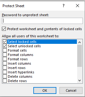
Enter a password in the ‘Password to unprotect sheet’ textbox. Any user will have to enter this to remove the sheet’s protection. The user can also decide what operations a person without the password may be allowed to do in the ‘Allow all users of this worksheet to’ list by scrolling down and selecting the specific checkboxes.

The options available are ‘Select locked cells’, ‘Select unlocked cells’, ‘Format cells’, ‘Format columns’, ‘Insert rows’, ‘Insert hyperlinks’, ‘Delete columns’, ‘Delete rows’, ‘Sort’, ‘Use AutoFilter’, ‘Use PivotTable and PivotChart’, ‘Edit objects, and ‘Edit scenarios’.

3. Click ‘ok’ once you are done.

All the cells in her sheet would have been protected according to the specifications she gave.

---

Protecting your Excel-Protecting Specific Cells in a Sheet

1. Select the cells you want locked by dragging by the fill handle.
2. Right click on your mouse after doing this. The following dropdown list will appear.

Click on ‘Format cells’ option. The following dialogue box will appear.

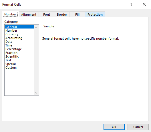
3. Click on the ‘Protection’ tab. You will find ‘Locked’ and ‘Hidden’ checkboxes. Uncheck ‘Locked’, which remains selected by default. Click ‘Ok’.
4. Now go to the ‘Review’ tab and select ‘Protect Sheet’.
5. Enter a password in the ‘Password to unprotect sheet’ textbox. Any user will have to enter this to remove the sheet’s protection. The user can also decide what operations a person without the password may be allowed to do in the ‘Allow all users of this worksheet to’ list by scrolling down and selecting the specific checkboxes.
6. Click on ‘Ok’ once done.

---

Protecting your Excel-Protecting a Specific Workbook

1. Click on the ‘Review’ menu and select ‘Protect Workbook’ option. The following dialogue box will appear.

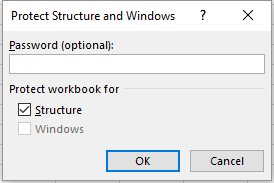
2. Enter your password and click on ‘Ok’.

---

Protecting your Excel-Allowing Certain Users to Edit Ranges in a Protected Spreadsheet

1. Select the ‘Review’ menu and click on ‘Edit Ranges’ option. The following dialogue box will appear.

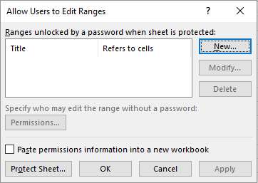
2. Click on the ‘New’ button. The following dialogue box will appear.
3. Enter a title in the ‘Title’ textbox.
4. Select the range of cells by pressing on the arrow near ‘Refers to cells’ textbox and then dragging or by entering manually in the textbox.
5. Enter a password in the ‘Range Password’ textbox.
6. Now select the ‘Permissions’ tab and add the users she wants to be able to edit in the ‘Group or usernames’ textbox.
7. Click on ‘Ok’ for all the subsequent dialogue boxes until completely done.

She can use any of these options to protect her sheet(s), according to her requirements and then by making sure that she shares her password with only her colleagues.