What is the LOOKUP Function?
LOOKUP Function in Excel scans through the given data in a range of cells to find the user a particular value that he or she wants. It is a worksheet function, meaning that, it can be used within a worksheet as a formula.
Where is the LOOKUP Function Found?
The LOOKUP function can be found in the ‘Formulas’ menu, under the group ‘Function Library’ as the part of a dropdown list by the name ‘Lookup & Reference’.
How to Use the LOOKUP Function?
The LOOKUP Function can be used in two different syntaxes, each of which we will look into in detail.
Syntax 1 – Vector Form
This form of the function searches for the value in a given range (called the lookup_range) and returns the value in the same range ( called the result_range).
Let us look at an example.
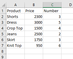
Sharon has the following data in her spreadsheet.
Syntax for the lookup function in the vector form is
LOOKUP( value, lookup_range, [result_range])
Parameters Description –
Value – is the particular data, information about which, we are trying to find.
Lookup Range – is the range of cells in which Excel is supposed to look for the value.
Result Range – is the range of cells in which Excel is supposed to look for its result (that is, the value in the result range corresponding to the value in the lookup range will be displayed as result)
Suppose, for the above data, Sharon wants to find out what costs 1500 out of all the products. For this, she should use the formula
=LOOKUP(1500, B1:B7, A1:A7).
Here, the result will appear as follows.
 Now, supposing Sharon wants to know which products she needs to arrange 6 pieces of, she can use the following formula
=LOOKUP( 6, C1:C7, A1:A7)
The result will appear as follows.

Syntax 2- Array Form
in the Array Form of the LOOKUP function, Excel looks for the data in the first row or column of the specified array and returns the result from the last column or row of the array.
Syntax for the LOOKUP function in Array syntax is as follows
= LOOKUP ( lookup_value, array)
Here, ‘look_up value’ is the data that Excel should search for and ‘array’ is the range of cells in which Excel should look for this value.
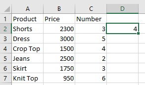
For the given data, suppose Sharon wants to know how many pieces are required for the product tat is priced at 1500. She can use the following formula
=LOOKUP (1500, B2:C7)
The result will appear as follows
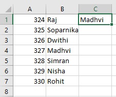
Now, in another situation, let us look at Rohan who comes across the following data.
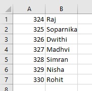
Rohan wants to know who is at Reference number 327 in the list. He can use the following formula
=LOOKUP(327, A1:B7)
The result will appear as follows