The Function Library of Excel has formulas that can come useful for any professional In this module we will look at two important financial functions necessary for a Financial Analyst.
Financial Functions – PMT
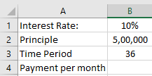
This function can be used to calculate the periodic loan payment that a person has to make. For example, Ridhi has the following sheet in which she has details for a loan that her client has taken. She can calculate the periodic payment for the client using this formula.
Syntax:
PMT(rate,nper,pv,[fv],[type])
Here,
‘Rate’ stands for the interest rate at which the payment is to be returned.
‘Nper’ stands for the total number of times the loaner has to pay to finish off his/her loan.
‘Pv’ stands for the principle or the present value.
‘Fv’ stands for Future Value. This is the amount that the loaner will have due after the payments have been made. This is optional and if the user does not enter it, it will be assumed to be zero.
‘Type’ stands for the payment that is due. For example, before the first payment, her type value will be 1 and after the last payment, her type value will be 0.
In the example above, the formula to be used is
=PMT(B1, B3, B2)
The results will appear as follows.
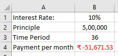 Please note that the result will appear as negative because this is an amount you have to pay from your side, that is, it is an amount that is going to be deducted from your bank account.
Alternatively, she can insert the same formula by going to the ‘Formulas’ menu, choosing the ‘Financial’ option in the ‘Function Library’ and selecting ‘PMT’ from the dropdown list that appears. The following dialogue box will appear.
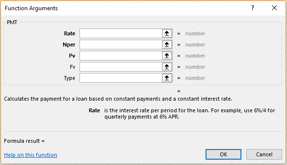
She can now enter the cell ranges or manually choose them by clicking on the arrow mark beside the textboxes and clicking ‘OK’.
Financial Functions – RATE
This function can be used to calculate the rate at which a person has to pay his/her interest, given the other details. For example, taking the same information as Ridhi’s but using it the other way round, we can try to see if we can reach the same result.
Syntax:
RATE(nper,pmt,pv,[fv],[type],[guess])
Here,
‘Nper’ stands for the total number of times the loaner has to pay to finish off his/her loan.
‘Pmt’ stand for the payment to be made every period.
‘Pv’ stands for the principle or the present value.
‘Fv’ stands for Future Value. This is the amount that the loaner will have due after the payments have been made. This is optional and if the user does not mention it, it will be assumed to be zero.
‘Type’ stands for the payment that is due. For example, before the first payment, her type value will be 1 and after the last payment, her type value will be 0.
‘Guess’ stands for the user’s guess of what the rate would be. It is assumed to be 10 if the user does not enter this value
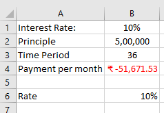
In the example above, the formula to be used is
=RATE(B3,B4, B2)
The results will appear as follows.
Alternatively, she can insert the same formula by going to the ‘Formulas’ menu, choosing the ‘Financial’ option in the ‘Function Library’ and selecting ‘RATE’ from the dropdown list that appears. The following dialogue box will appear.
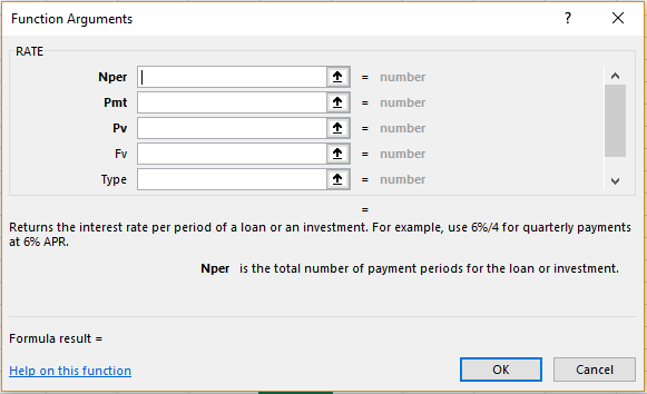
She can now enter the cell ranges or manually choose them by clicking on the arrow mark beside the textboxes and clicking ‘OK’.