Linear regression with one variable
Model representation
In supervised learning we have a data set and this data set is called a training set.For example housing prices example we have a training set of different housing prices and our job is to learn from this data how to predict prices of the houses.
Let us define some notation that we will use for representation:
m = Number of training examples we have
x’s = input variables/features [in housing price example we have size as input variable]
y’s = output or target variables [in housing price example we have price as output variable]
So we have (x,y) as a one training example.To refer to the specific example let’s say for i’th example we can write
(x^(i), y^(i)) [This i in the parenthesis is not the exponentiation,but that is just an index into our training set and refers to the i’th row in training set table]
We can describe supervised learning diagrammetically as following:
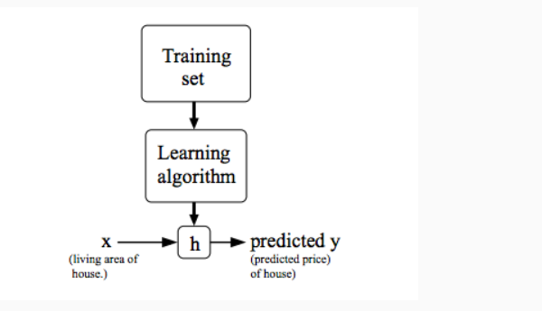
In supervised learning our main goal is, given a training set, we have to learn a function h : X → Y so that if h(x) is a “good” predictor for the corresponding value of y or not.This function h is called hypothesis.In linear regression with one variable we have hypothesis as:
hθ(x)=θ0+θ1(x) where θ0,θ1 are parameters
Cost Function
This cost function will let us figure out how to fit the best possible straight line to our data.Cost function is used to measure the accuracy of our hypothesis function.Cost function will take an average difference of all the results of the hypothesis with inputs from x’s and the actual output y’s.
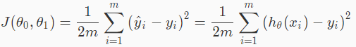
This cost function is also called the “Squared error function”, or “Mean squared error”. When we compute gradient descent, the derivative term of the square function will cancel out the (1/2) term,so for convenience the mean in the cost function is halved(1/2).The following image will tell us in short what the cost function does:
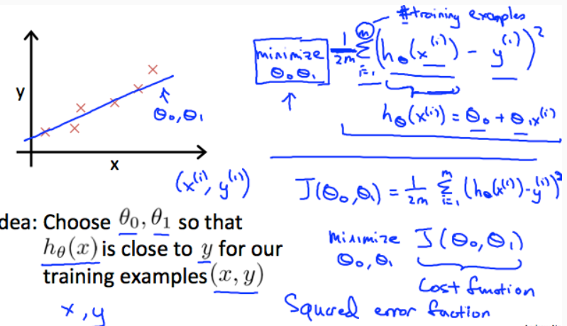
Thus our main goal is that we should try to minimize the cost function.
Gradient descent
Gradient descent is the algorithm for minimizing the cost function.It is the more general algorithm,not only used in linear regression,but used in all over places in machine learning.
The gradient descent algorithm is writtern as following:
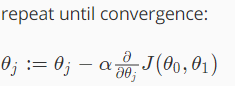
where j = 0,1 represent the attributes’s index number.
In the gradient descent algorithm. α is the learning rate which represent how big a step we take when updating our parameter θj
We should simultaneously update the parameters θ1,θ2,...,θn at each iteration j. If we will update a specific parameter prior to calculating another one on j’th interation like we calculate θ0 and update it and after that we again calculate θ1 then it would yield a wrong implementation.
If the value of α is too small in our model then gradient descent can be slow and if the value of α is too large in our model then gradient descent can overshoot the minimum.
It may fail to converge or even diverge.
This is all about model representation, hypothesis function, cost function and algorithm to minimize the cost function(called gradient descent) in machine learning field.