After we are done with an Excel sheet, there maybe a need for highlighting cells that are important. In this article, we will look at how we can do this.
- Greater Than
- Less Than
- Between
- Equal to
- Text that Contains
- Date occurring
- Duplicate Values
Highlighting cells-Greater Than
This option can be used if we want to highlight cells that have values greater than a particular value.
To do this, select the ‘Home’ menu and then click on ‘Conditional Formatting’ from the ‘Styles’ group. A dropdown list as follows will appear.
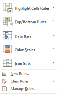 Now click on ‘Highlighting Rules’ to display another dropdown list.
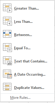 Choose ‘Greater Than’. A dialogue box will appear.
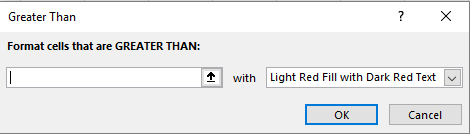 Enter the value, greater than which, the cells should be highlighted in the ‘Format cells that are GREATER THAN’ text box. You can choose the colour of your highlight in the list beside the textbox.
Press ‘OK’ once you are done.
Highlighting cells-Less Than
This option can be used if we want to highlight cells that have values lesser than a particular value.
To do this, select the ‘Home’ menu and then click on ‘Conditional Formatting’ from the ‘Styles’ group. A dropdown list will appear. Now click on ‘Highlighting Rules’ to display another dropdown list. Choose ‘Less Than’ from this and a dialogue box will appear.
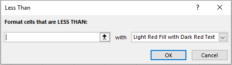
Enter the value, lesser than which, the cells should be highlighted in the ‘Format cells that are LESSER THAN’ text box. You can choose the colour of your highlight in the list beside the textbox.
Press ‘OK’ once you are done.
Highlighting cells-Between
This option can be used if we want to highlight cells that have values between two particular values.
To do this, select the ‘Home’ menu and then click on ‘Conditional Formatting’ from the ‘Styles’ group. A dropdown list will appear. Now click on ‘Highlighting Rules’ to display another dropdown list. Choose ‘Between’ from this and a dialogue box will appear.
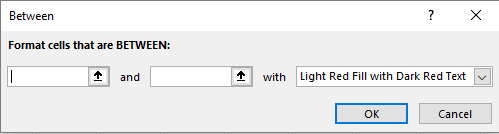
Enter the values, between which, the cells should be highlighted in the ‘Format cells that are BETWEEN’ text boxes. You can choose the colour of your highlight in the list beside the textboxes.
Press ‘OK’ once you are done.
Highlighting cells-Equal To:
This option can be used if we want to highlight cells that have values equal to a particular value.
To do this, select the ‘Home’ menu and then click on ‘Conditional Formatting’ from the ‘Styles’ group. A dropdown list will appear. Now click on ‘Highlighting Rules’ to display another dropdown list. Choose ‘Equal to’ from this and a dialogue box will appear.
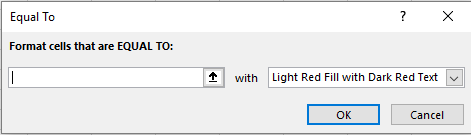
Enter the value, equal to which, the cells should be highlighted in the ‘Format cells that are EQUAL TO’ text box. You can choose the colour of your highlight in the list beside the textbox.
Press ‘OK’ once you are done.
Highlighting cells-Text that Contains:
This option can be used if we want to highlight cells that have text that contains a particular word.
To do this, select the ‘Home’ menu and then click on ‘Conditional Formatting’ from the ‘Styles’ group. A dropdown list will appear. Now click on ‘Highlighting Rules’ to display another dropdown list. Choose ‘Text that contains’ from this and a dialogue box will appear.
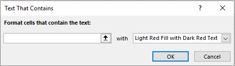
Enter the text, containing which, the cells should be highlighted in the ‘Format cells that contain the text’ text box. You can choose the colour of your highlight in the list beside the textbox.
Press ‘OK’ once you are done.
Highlighting cells-Date Occurring:
This option can be used if we want to highlight cells that have date occurring at a particular time.
To do this, select the ‘Home’ menu and then click on ‘Conditional Formatting’ from the ‘Styles’ group. A dropdown list will appear. Now click on ‘Highlighting Rules’ to display another dropdown list. Choose ‘Date Occurring’ from this and a dialogue box will appear.
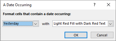
Select the day, which contain the dates that should be highlighted in the ‘Format cells that contain a date occurring’ list. You can choose the colour of your highlight in the list beside the textbox.
Press ‘OK’ once you are done.
Highlighting cells-Duplicate Values:
This option can be used if we want to highlight cells that have duplicate values.
To do this, select the ‘Home’ menu and then click on ‘Conditional Formatting’ from the ‘Styles’ group. A dropdown list will appear. Now click on ‘Highlighting Rules’ to display another dropdown list. Choose ‘Duplicate Values’ from this and a dialogue box will appear.
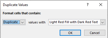
Choose if duplicate/unique values should be highlighted in the ‘Format cells that contain’ list. You can choose the colour of your highlight in the list beside the textbox.
Press ‘OK’ once you are done.
Example:
Sonam wants to highlight all the cells that contain ‘3’ in it. How can she do it?
Solution:
To do this, she should select the ‘Home’ menu and then click on ‘Conditional Formatting’ from the ‘Styles’ group. A dropdown list will appear. She should now click on ‘Highlighting Rules’ to display another dropdown list and choose ‘Text that contains’ from this and a dialogue box will appear. She should then enter ‘3’ in the ‘Format cells that contain the text’ text box and press ‘OK’ once done.