One of the most desirable features of the Microsoft Excel Spreadsheet is that one can customize it according to the needs and purposes of one’s organization. This article is about the different ways in which one may do the Customization in Excel.
Following is a list of various customizing features available in Microsoft Excel:
- Changing the colour theme
- Customization of one’s ribbon
- Formula Settings
- Proofing
Each one of these are discussed in detail in the following sections.
Changing the Color Theme – Customization in Excel
Step 1: Click on the ‘File’ menu on the ribbon. Now, select the ‘Options’ button. You can find it on the lowermost end of the green bar found on the left.
Step 2: The ‘Excel Options’ dialogue box is expected to appear. By default, the ‘General’ option will remain selected. Do not change this.
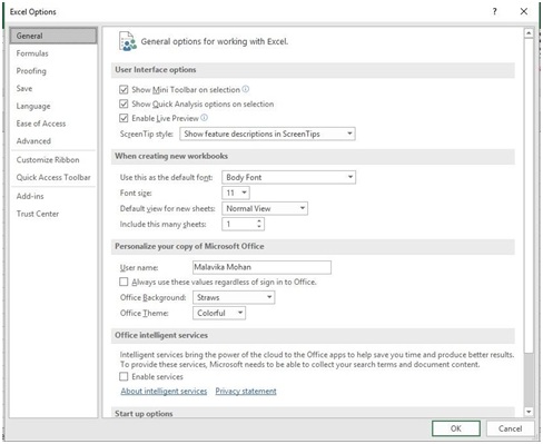
Under the heading ‘Personalize your copy of Microsoft’, one can find the ‘Office Theme’ dropdown list. It contains three options- Colourful, Dark Grey and White.
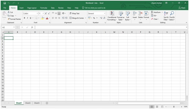
Colorful Theme
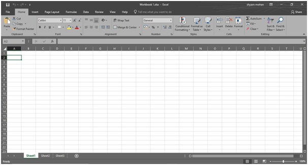
Dark Grey Theme
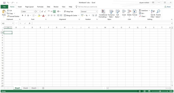
White Theme
Step 3: Choose the option that you like the most and click on the ‘Ok’ button once you are done.
You have now changed the colour theme of your Microsoft Excel Spreadsheet according to your wish.
Customization of One’s Ribbon
To customize the ribbon, you can either delete tabs you do not want or include new tabs.
Deleting a Tab
Step 1: Click on the ‘File’ menu on the ribbon. Now, select the ‘Options’ button. You can find it on the lowermost end of the green bar found on the left.
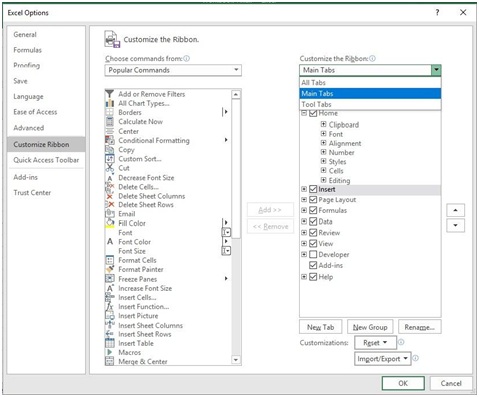
Step 2: The ‘Excel Options’ dialogue box is expected to appear. By default, the ‘General’ option will remain selected. Click on the ‘Customize Ribbon’ option found a few options below ‘General’.
You will find two dropdown lists. The ‘Choose Commands From’ dropdown list on the left and the ‘Customize Your Ribbon’ dropdown list on the right. Ignore the former and go to the “Customize Your Ribbon’ dropdown list.
This dropdown list has three options- All Tabs, Main Tabs and Tool Tabs.
‘All Tabs’ will show you all the tabs that are present in the ribbon. This list is very long and maybe cumbersome and time consuming to deal with.
‘Main Tabs’ will show you the major menus on the ribbon, using which is usually enough to customize an average user’s spreadsheet.
The ‘Tool Tabs’ option will show you the tabs that are specifically used for designing and formatting various content like pictures, drawing, SmartArt, etc.
Choose the option that best suites you.
Step 3: Each option in the dropdown list will have small checkboxes near it that remain selected. Unselect these for the tabs that you do not wish to appear on your ribbon.
Step 4: Click on the ‘Ok’ button once you are done.
Including a New Tab in the Ribbon
Step 1: Click on the ‘File’ menu on the ribbon. Now, select the ‘Options’ button. You can find it on the lowermost end of the green bar found on the left.
Step 2: The ‘Excel Options’ dialogue box is expected to appear. By default, the ‘General’ option will remain selected. Click on the ‘Customize Ribbon’ option found a few options below ‘General’.
You will find two drop down lists. The ‘Choose Commands From’ dropdown list on the left and the ‘Customize Your Ribbon’ drop down list on the right. Ignore the former and go to the “Customize Your Ribbon’ dropdown list.
This drop down list has three options- All Tabs, Main Tabs and Tool Tabs.
‘All Tabs’ will show you all the tabs that are present in the ribbon. This list is very long and maybe cumbersome and time consuming to deal with.
‘Main Tabs’ will show you the major menus on the ribbon, using which is usually enough to customize an average user’s spreadsheet.
The ‘Tool Tabs’ option will show you the tabs that are specifically used for designing and formatting various content like pictures, drawing, SmartArt, etc.
Choose the option that best suites you.
Step 3: Click on the ‘New Tab’ button below the drop down list. A ‘New Tab’ will appear in the drop down list.
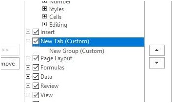
Step 4: Now click on the new tab that you have just created and right click. Click on the ‘Rename’ option from the drop down list. Enter a name of your choice for the tab.
Step 5: Right click on the ‘New Group’ option below it and choose ‘Rename’. Give it a name of your choice. You can add commands to this new tab you have just created by selecting the suitable options from the drop down list on the left namely ‘Choose commands from’.
Step 6: Click on the ‘Add’ button. Press ‘Ok’ once you are done.
You have now customized your ribbon.
Formula Settings in Excel
Each person has a different need of formula setting according to their purpose.
To change the formula settings for your spreadsheet, do as follows:
Step 1: Click on the ‘File’ menu on the ribbon. On the green bar on the left, select ‘Options’, which is found on the lowermost part.
The ‘Excel Options’ dialogue box is expected to appear.
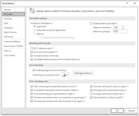
Step 2: By default, the ‘General’ option remains selected. Click on the ‘Formulas’ option just below it. This will show you the various options for formulas under four headings: Calculation Options, Working with Formulas, Error Checking and Error Checking Rules.
‘Calculation Options’ various options for calculating the results for the formula like whether or not it has to be performed manually by the user or done automatically, etc.
‘Working with Formulas’ gives you various options that make operating easier. You can decide to use or not use R1C1 reference style or let excel complete the formula for you after you just enter the beginning of it (Formula AutoComplete), etc.
‘Error Checking’ lets you decide whether or not you would like your user to be warned when an error has been entered, and in which colour this should be indicated.
‘Error Checking Rules’ is an elaboration on the last option that gives you various rules by which a data is interpreted as error or not by Excel.
The user can find small check boxes against all of these options and select them if they want that option to be functional and unselect them if not.
Proofing in Excel
Proofing is basically to check the language used for data entry in the Excel sheet.
Step 1: Click on the ‘File’ menu on the ribbon. On the green bar on the left, select ‘Options’, which is found on the lowermost part.
The ‘Excel Options’ dialogue box is expected to appear.
Step 2: By default, the ‘General’ option remains selected. Click on the ‘Proofing’ option below.
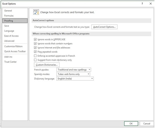
The user has various options
- If Excel should keep changing the data a user enters as and when it is typed using the AutoCorrect option
- Whether or not to ignore text when entered in uppercase
- Whether or not to ignore words that contain numbers
- Whether or not Excel should ignore website links and file addresses
- Whether or not Excel should mark the words that keep getting repeatedly used
- Whether or not Excel should use accented uppercase for data in French
- Whether or not Excel should suggest words only from the dictionary specified.
The user can select the check boxes that he/she wishes to keep and click ‘Ok’ once done.These are some of the ways in which a user can customize his/her spreadsheet to add individuality to it.