What is Conditional Formatting?
Conditional Formatting is an option available in Excel that allows one to highlight the trends in a range. Doing this will help one spot important and necessary values easily.
Where is the Conditional Formatting option Present?
It can be found in the ‘Styles’ group of ‘Home’ menu in an Excel sheet.
How to Create a Conditional Formatting Rule?
Sera has a spreadsheet for which she wants to use conditional formatting to highlight cells that are greater than 1000.
To create a new Conditional Formatting Rule, select the range of cells containing the data and then click on the ‘Conditional Formatting’ option. The following dropdown list will appear.
 The various options in this list are as follows.
Highlight Cell Rules:
This option will highlight the cells that fits into a particular criteria. The available criterion are ‘Greater Than’, ‘Less Than’, ‘Between’, ‘Equal to’, ‘Text That Contains’, ‘A Date Occurring’ and ‘Duplicate Values’.
Greater Than: This option can be used to format cells that contain value that are more than a given one.
Less Than: This option can be used to format cells that contain value that are less than a given one.
Between: This option can be used to format cells that contain value that are between two given values.
Equal to: This option can be used to format cells that contain value that are equal to a given one.
Text That Contains: This option can be used to format cells that contain a certain text.
A Date Occurring: This option can be used to format cells that contain a date that occurs during a specific period.
Duplicate Values: This option can be used to format cells that contain duplicate values.
Once she selects one of these criterion, a dialogue box as follows will appear.
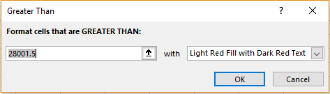 She can enter ‘1000’ in the ‘Format cells GREATER THAN’ textbox and choose the colour in the second one. Click ‘Ok’ once done.
Top/Bottom Rules:
This option can be used to format cells that are the least or most of a given criteria. The various available criterion are ‘Top 10 items’, ‘Top 10%’, ‘Bottom 10 items’, ‘Bottom 10%’, ‘Above Average’ and ‘Below Average’.
Top 10 items: This will format cells that have the top ranks in the given table. Though the option says ’10’ it is valid for any number.
Top 10 %: This will format cells that have the top percentages in the given table. Though the option says ’10’ it is valid for any number.
Bottom 10 items: This will format cells that have the bottom ranks in the given table. Though the option says ’10’ it is valid for any number.
Bottom 10 %: This will format cells that have the bottom percentages in the given table. Though the option says ’10’ it is valid for any number.
Above Average: This will format cells that are above the average value in the given table.
Below Average: This will format cells are below the average value in the given table.
Upon choosing one of these, the following dialogue box will appear.
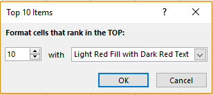 Here, she can choose how many ranks from the top she wants to format from the list given. She can also choose the colour of highlight in the adjacent list.
Data Bars:
This option will create bars for the value entered in each cell for its specific value. The options available are ‘Gradient Fill’ and ‘Solid Fill’.

Gradient Fill: This will show bars that have fading colourings.
Solid Fill: This will show bars that have opaque colourings.
Icon Sets:
This option allows her to include icons that are representative of the data in each cell.
The various options available under these are ‘Directional’, ‘Shapes’, ‘Indicators’ and ‘Ratings’.
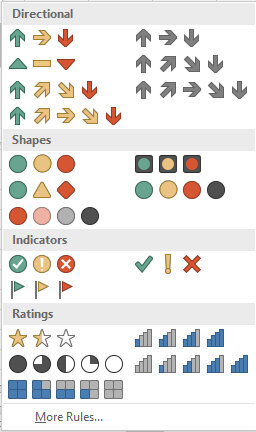 Directional: This shows arrow marks pointing in various directions and is useful to show if a trend is increasing or decreasing.
Shapes: These have different coloured shapes and can be used to indicate positivity and negativity of values using the colours.
Indicators: These have different indicators and can be used to indicate positivity and negativity of values using ticks, crosses, etc. respectively.
Ratings: This can be used to show the opinion of someone on a given data using stars, bars, etc.
She can choose the option that best suits her needs.
Editing Conditional Formatting
After Sera has formatted her cells, she now wants to edit the formatting to highlight cells that satisfy a certain formula. She can do this by clicking on the range, the formatting for which she wants to change and then clicking on the ‘Conditional Formatting’ option. From the dropdown list, she can choose ‘Manage Rules’. The following dialogue box will appear.
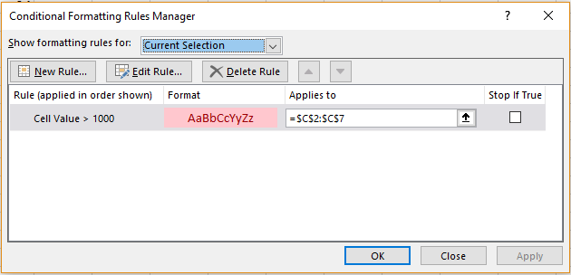
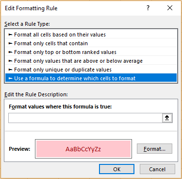
She can now select the formatting rule she wants to edit and click on the ‘Edit Rules’ option. She can change the Rule type to ‘Use a formula to determine which cells to format’ option and enter the formula in ‘Format cells where this formula is true’ textbox. Click ‘Ok’ once done.
Adding a New Rule to Conditional Formatting
Suppose Sera wants to add a new condition to her formatting, she can do this by clicking on the ‘Conditional Formatting’ option from the ‘Styles’ group in the ‘Home’ menu and click on the ‘Manage Rules’ option. From the dialogue box, she can click on the ‘New Rule’ option and select the new condition from the given options.
Removing Conditional Formatting
Sera has added her conditional formatting but her boss wants her to give her a sheet that does not have any of this. For this now, she has to remove this formatting. How will she do it? She can do this by selecting a cell that has been formatted and clicking on the ‘Conditional Formatting’ option from the ‘Styles’ group of ‘Home’ menu. From the dropdown list, she can choose ‘Clear Rules’ option. She can either choose ‘Clear Rules from Selected Cells’ to remove formatting for only the cells she has clicked on or ‘Clear Rules from the Entire Sheet’ to remove all formatting from the sheet.