What are Sparklines in Microsoft Excel?
Sparklines in Microsoft Excel are small chart like figures that provide a summary of the data, visually, in a cell.
Why Use Sparklines in Microsoft Excel?
Sparklines can be used to show a recurring pattern in values like increasing or decreasing, periodic economic cycles or even simply to emphasize on the maximum or minimum values.
Where to Find ‘Sparklines’ in Microsoft Excel?
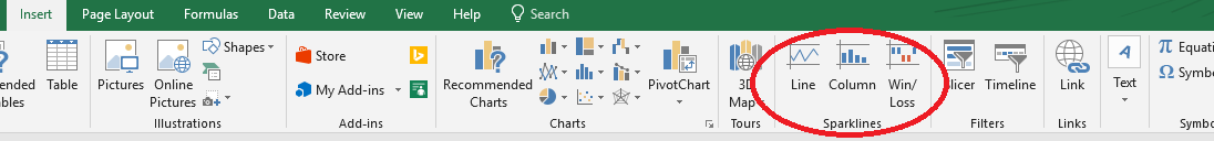
The ‘Sparklines’ group of cells is present in the ‘Insert’ menu towards the right hand side.
What are the Different Types of Sparklines in Microsoft Excel?
The different types are:
- Line Sparkline
- Column Sparkline
- Win/Loss Sparkline
How to Insert ‘Sparklines’ in Microsoft Excel?
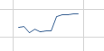
- Line Sparkline: A Line Sparkline will show the data as small charts for each cell as rows.
Step 1: Select the cells you want the Sparkline charts to be made for by dragging and click on the ‘Insert’ tab and then the ‘Line’ option in the ‘Sparklines’ grouping. The following dialogue box will appear.
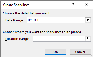
Step 2: Enter a range where you would like the Sparklines to be displayed in the ‘Location range’ textbox. Click ‘Ok’.
Step3: The ‘Design’ tab will open itself on the top where you can change the appearance of the sparklines.
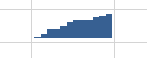
2. Column Sparkline: A Column Sparkline will show the data as small charts for each cell as columns.
Step 1: Select the cells you want the Sparkline charts to be made for by dragging and click on the ‘Insert’ tab and then the ‘Column’ option in the ‘Sparklines’ grouping. The same dialogue box as before will appear.
Step 2: Enter a range where you would like the Sparklines to be displayed in the ‘Location range’ textbox. Click ‘Ok’.
Step3: The ‘Design’ tab will open itself on the top where you can change the appearance of the sparklines.
3. Win/Loss Sparkline: A Win/Loss Sparkline will show the data as small charts for each cell as a comparison.
Step 1: Select the cells you want the Sparkline charts to be made for by dragging and click on the ‘Insert’ tab and then the ‘Win/Loss’ option in the ‘Sparklines’ grouping. The same dialogue box as before will appear.
Step 2: Enter a range where you would like the Sparklines to be displayed in the ‘Location range’ textbox. Click ‘Ok’.
Step3: The ‘Design’ tab will open itself on the top where you can change the appearance of the sparklines.
Example:
Sunaina wants to make a sparkline for her company’s monthly report as follows. She wants them to look row-like. How can she do it?
Solution:
She should select the cells she wants the Sparkline charts to be made for by dragging and click on the ‘Insert’ tab and then the ‘Line’ option in the ‘Sparklines’ grouping. A dialogue box will appear.She should then enter a range where you would like the Sparklines to be displayed in the ‘Location range’ textbox. Click ‘Ok’.