Slicers are advanced filtering features available in Excel which can be used for table and Pivot Table data entries. When you use Slicers, Excel shows you the current filtering in use and filters the values according to the criteria given.
In this module, we will look at the following:
- Creating a Slicer
- Components of a Slicer
- Formatting a Slicer
- Deleting a Slicer
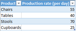
Roshan has a table of the various products that his company manufactures and their production rate. This data is shown as follows
Creating a Slicer
To create a slicer for his table, Roshan should click on any cell in the table and select the ‘Insert’ menu. Here, he can choose the ‘Slicer’ option from the ‘Filters’ group. The following dialogue box will appear.
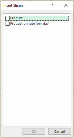 He can check the box near the heading, the options under which he wants to add Slicer. he should click ‘Ok’ once done.
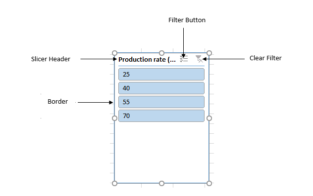
The data will appear as follows.
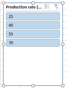 Clicking on any of these options will display him the details corresponding to that value and he can easily filter the value that he wants.
Components of a Slicer
Now that he has inserted a Slicer, it is important to know the various parts of this and understand their functions. These are as follows
Slicer Header: This option shows the title of the slicer and hints him about the contents present in it.
Filter Button: If this button is selected, it shows that the item is included in the filter and vice versa if it is not.
Clear Filer: This button removes all the filtering of the item.
The moveable and resizable border enables you to change the size and location of the Slicer.
Formatting a Slicer
To change the look of a slicer, he should select the Slicer that he wans formatted and click on the ‘Slicer Tools – Options’ tab and choose the one he desires from the ‘Slicer Styles’ option.
Deleting a Slicer
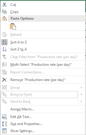
To delete the Slicer, he has to right-click on the Slicer he wants to delete and from the dropdown list that appears, select ‘Remove Slicer “Production rate per day”‘.
The Slicer will be deleted.
