Text functions are those predefined formulae available on Excel that can be used on alphabetical characters or strings. In this module we will look at CODE and CHAR functions.
Text Functions – CODE
This function can be used to display a specific numerical value to an alphabetical character. This character is decided by the character set that is stored in our computer. The code assigned is corresponding to the ASCII code for the character.
Syntax:
CODE(text)
Here, ‘text’ corresponds to the cell reference, the first alphabet of the data contained in which, needs to be assigned a code.
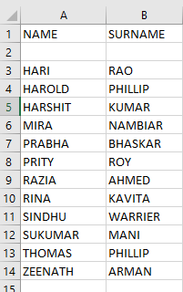
Fathima High School is having an exam for its Class 12 students in the coming month. Each student is going to be assigned a confidential code for ensuring unprejudiced and unbiased correction by the teachers. The code consists of two parts: One having a number that corresponds to the first letter of their name and the other to their surname. The details are given as below.
To insert the identification code, the management can use the CODE function. The formula they should use is
=CODE(A3)
=CODE(B3)
They can now extend this function to the rest of the cells by dragging. The result will appear as follows.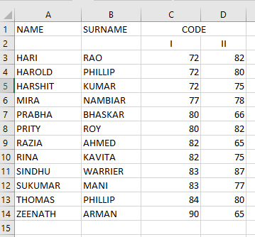
Another way to insert this function is by going to the ‘Function Library’ in the ‘Formulas’ menu and clicking on the CODE option from ‘Text’ dropdown list. The following dialogue box will appear.
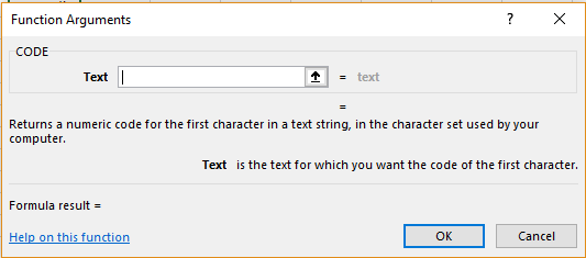 They can enter the cell reference in the ‘Text’ textbox and then click ‘OK’.
Text Functions – CHAR
After the evaluation is done, the management now wants to return the codes as names. The teachers have handed over the following sheet.
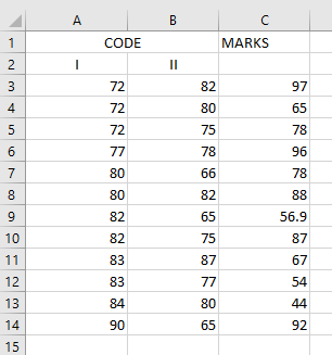
To decode these, they can use the CHAR function. This will return the characters that were coded by CODE function before, according to the number system followed by the computer. The code is decoded according to the ASCII table.
Syntax:
CHAR(text)
Here, text corresponds to the cell reference that contains the code to be decoded.
The formulae they should use are
=CHAR(A3)
=CHAR(B3)
and extend it for the rest of the rows by dragging. The result will appear as follows.
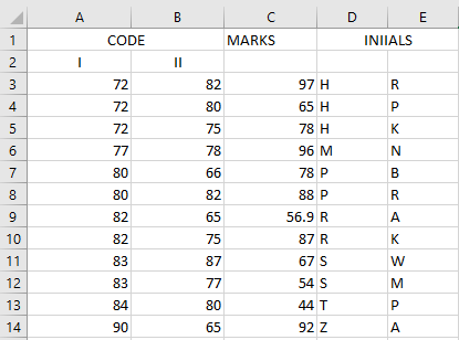 All they have to now do is compare these list of initials with the student list of Class 12.
Another way to insert this function is by going to the ‘Function Library’ in the ‘Formulas’ menu and clicking on the CHAR option from ‘Text’ dropdown list. The following dialogue box will appear.
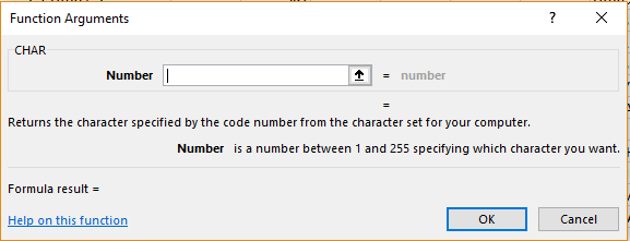
They can enter the cell reference in the ‘Number’ textbox and then click ‘OK’.