An Advanced filter can be used in Excel to filter data with criteria. Shayne has some data that he would like to filter to obtain details of just the employees from UK. Here is how he can do it.
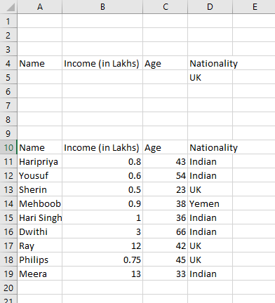
To do this, he should set a criteria above the data to be filtered. He should use labels as the same used in the table, in the same order and specify the desired detail. An example is shown below.
 He should now click on the ‘Advanced’ option in the ‘Sort & Filter’ group in the ‘Data’ menu.
The following dialogue box will appear.
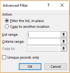 If he would like to filter the list in its current place, he can use the ‘Filter the list, in-place’ option.If he wants to copy the list to somewhere else and then filter the data, he select the ‘Copy to another location’ option.
After this, he can select the range where the data is present by using the arrow near ‘List Range’ textbox. He can select the range where the criteria is present by using the arrow near the ‘Criteria Range’ textbox. In case he has chosen the second option to copy the list to another location, he can select this range where the data should be copied to in the ‘Copy to:’ textbox by using the arrow beside it.
He can check the ‘Unique records only’ checkbox to avoid repetitions. Click ‘Ok’ once done.
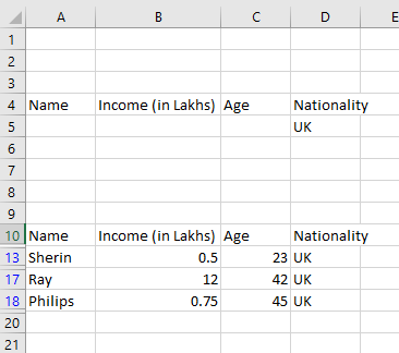
The filtered data will appear as follows.
 AND Criteria
Suppose he has two criteria and wants to display the results that match both, he can use the AND criteria.
For example, he wants to display the people who are from UK and aged 23, he can use the criteria as follows.
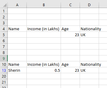
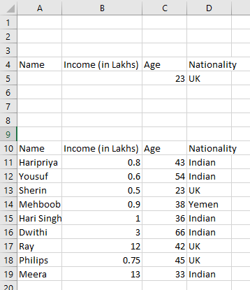 Now, he should click on the ‘Advanced’ option from the ‘Sort & Filter’ group and has to include this cell as well in the range of cells for the ‘Criteria range:’ textbox. ‘List Range’ will remain the same. After clicking ‘Ok’, the filtered data will appear as follows:
 OR Criteria
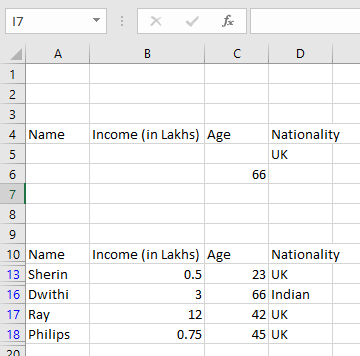
Now, suppose Shayne wants to view the details of employees who are from UK or aged 66, he can be do this as follows. He should enter ‘UK’ under ‘Nationality’ column in the first row under the label. He should then enter ’66’ under the ‘Age’ label in the row below. As follows,
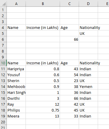 Going to the ‘Advanced’ option in the ‘Sort & Filter’ group of the ‘Data’ tab, he should include these cells in the ‘Criteria Range:’ textbox as well. The ‘List Range:’ will remain the same. Once he presses ‘Ok’, the results will appear as follows:
