V LOOKUP and H LOOKUP are important functions in Excel that can be used for finding values in an Excel sheet. This article will explain about the various provisions provided by both.
V LOOKUP in Excel
V LOOKUP or Vertical Lookup is a worksheet function that helps a user search for a given piece of information in the columns of a sheet.
Sreekar has the following sheet.
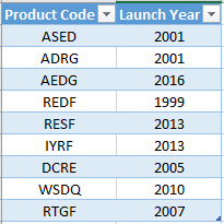
He wants to know in which year the product with code ADRG was launched. He can use this function to look for this data.
Syntax:
VLOOKUP( lookup_value, table_array,col_index_num,[range_lookup])
Where,
lookup_value – refers to the value in relation to which the new value has to be found.
table_array – refers to the range in which the data is present.
col_index_num – refers to the column number where the result can be found.
range_lookup – can be used to specify if the matching should be approximate or exact. If ‘TRUE’ is entered, the function will return an approximate output and ‘FALSE’ will return an exact output.
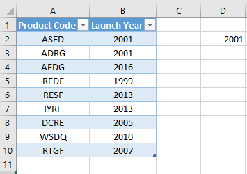
The formula Sreekar should use is
=VLOOKUP("ADRG",A1:B10,2,FALSE)
The result will appear as follows.
Alternatively, he can go to the ‘Formulas’ tab and click on the ‘Lookup & Reference’ option. From the dropdown list he can choose ‘VLOOKUP’. The following dialogue box will appear. He can enter the cell references or manually select these using the arrow mark near the text box.
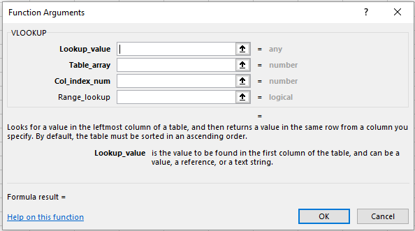
Click ‘OK’ once done.
H LOOKUP in Excel
H LOOKUP or Horizontal Lookup is a worksheet function that helps a user search for a given piece of information in the rows of a given sheet.
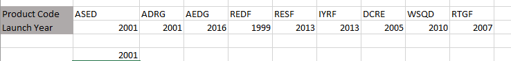
Suppose in the given sheet was horizontal as follows and he wants to look for the same data, he can use this formula.
![]()
Synatx:
HLOOKUP( lookup_value, table_array,row_index_num,[range_lookup])
Where,
lookup_value – refers to the value in relation to which the new value has to be found.
table_array – refers to the range in which the data is present.
row_index_num – refers to the row number where the result can be found.
range_lookup – can be used to specify if the matching should be approximate or exact. If ‘TRUE’ is entered, the function will return an approximate output and ‘FALSE’ will return an exact output.
The formula he should use is = HLOOKUP("ADRG",A1:J2,2,FALSE)
The result will appear as follows.
Alternatively, he can go to the ‘Formulas’ tab and click on the ‘Lookup & Reference’ option. From the dropdown list he can choose ‘HLOOKUP’. The following dialogue box will appear. He can enter the cell references or manually select these using the arrow mark near the text box.
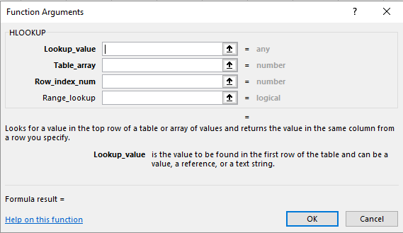 Click ‘OK’ once done.