Druva has a Pivot Table consisting of her expenses for April and May. It looks as follows
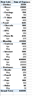
In this module, we will look at the advanced features that she can use to modify this table.
- Inserting Timelines
- Creating Pivot Charts
- Formatting and Customizing Pivot Table
Inserting Timeline
By inserting a timeline, she can filter the data in her Pivot Table according to various time periods. These are modified forms of slicers.
To insert a timeline to the table, one should make sure that there is a date feature available in it. As it is in the example shown above, this can be inserted easily. To do this, she should select the table and click on ‘Timeline’ option in the ‘Filters’ group of ‘Insert’ menu. The following dialogue box will appear.
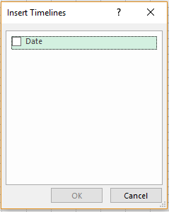 She should check the box beside ‘Date’ and click the ‘OK’ button.
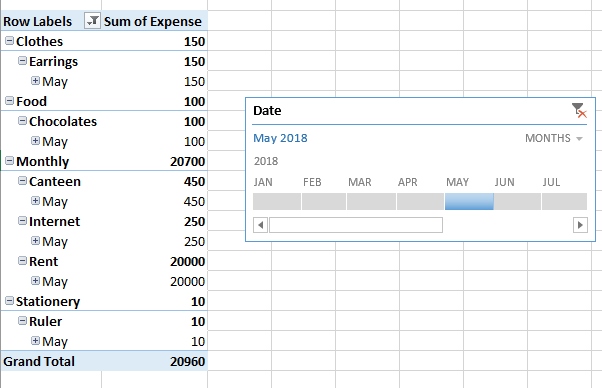
The timeline will appear as follows.
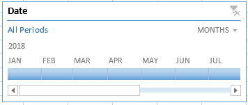 In the dropdown list above (Which now has ‘MONTHS’ written) she can select if she wants to view the timeline as years, months, quarters or days. Now, if she clicks on one of these options, the Pivot Table will be filtered to show her the results corresponding to the particular time.
For example, suppose she chooses ‘May’ from this timeline, the result will appear as
Creating Pivot Charts
While Pivot Tables summarize the complex data in a tabular format, a Pivot Chart does the same in a graphical form.
To insert a Pivot Chart, she should select the table and then click on the ‘Pivot Chart’ option and click on the ‘Pivot Chart’ option from the dropdown list in the ‘Charts’ group of ‘Insert’ menu. The following dialogue box will appear.
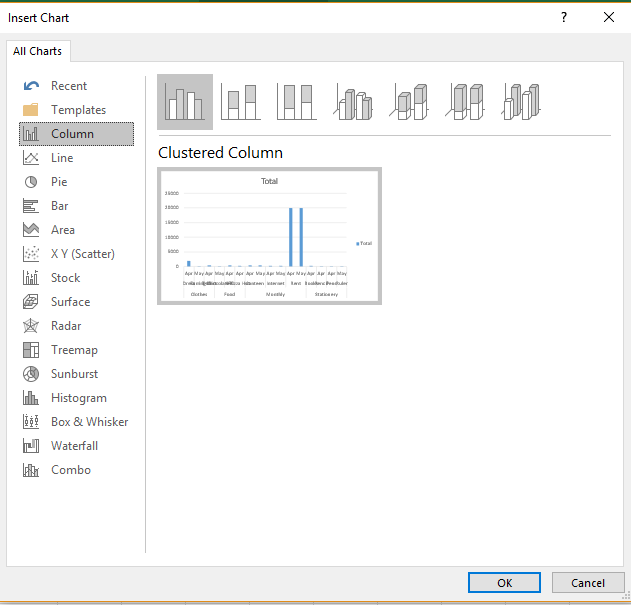 She can choose the chart style she wants from the options given on the left and click ‘Ok’ once done. The chart will be inserted.
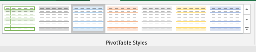
Formatting and Customizing Pivot Table
To format the Pivot Table, she should click on the table and select the ‘Pivot Tables- Design’ tab. Now, in ‘Pivot Table Style Options’ she has following options.
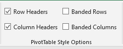
Row Headers: The box will remain checked if her Pivot Table has headings for rows. She can uncheck it if she doesn’t want this.
Column Headers: The box will remain checked if the table has headings for columns. She can uncheck it if she doesn’t want this.
Banded Rows: If she checks this option, her Pivot Table will have horizontal bands in the background.
Banded Columns:If she checks this option, her table will have vertical bands in the background.
If she wants to change the look of the table, she can do this by choosing a suitable one from the options given under ‘Pivot Table Styles’. All she has to do is click on the table and then click on the style she wants.