Information Functions can be used when one deals with important data. Two important functions in this category are CELL and ERROR.TYPE. We will look at these in detail in this article.
Information Functions – CELL
This function can be used to return the information of the cell one is entering in.
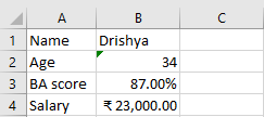
For example, Sreya has the following sheet. She has to mention the kind of formatting she has used for each row at the end of the row so that Sravan can make a sheet just like hers. To do this, she can use the CELL function.
Syntax:
=CELL(information,[reference])
Here, ‘information’ refers to the type of information that needs to be displayed. The options available are as follows:
- address
- col
- color
- contents
- filename
- format
- parentheses
- prefix
- protect
- row
- type
- width
‘Reference’ option is an optional entry that can be used to include the cell reference of the cell you want to display information about.
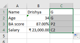
The formula she can use is
=CELL(“format”,B1) and drag it to the rest of the cells of the row.
the result will appear as follows
 Alternatively, she can go to the ‘Function Library’ in ‘Formulas’ tab and choose ‘More Functions’. Here she should choose ‘Information’ and then ‘CELL’. The following dialogue box will appear.
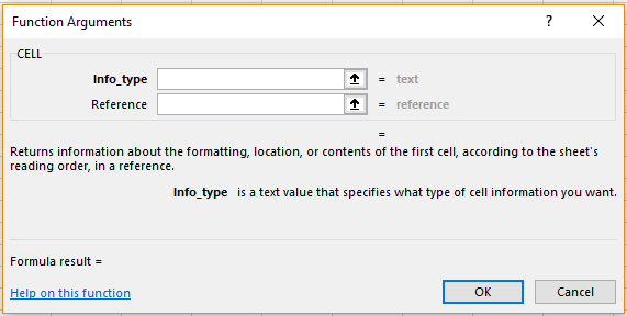
She can give the necessary details and click ‘OK’ to proceed.
Information Functions – ERROR.TYPE
This function can be used to return a particular value instead of displaying error on Excel.
For example, in the sheet that Sreya was using, she enters a function wrong and the error displayed is as ‘#NAME?’.
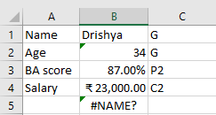
She wants to replace this with a value. She can do this using this function.
Syntax:
=ERROR.TYPE(error_value)
Here, ‘error_value’ refers to the number to be displayed in case of error. The error types and their subsequent values are as follows:
- #NULL! – 1
- #DIV/0 – 2
- #VALUE! – 3
- #REF! – 4
- #NAME? – 5
- #NUM! – 6
- #N/A – 7
- #GETTING_DATA – 8
- All other errors – N/A
To display her error as a value, she can use the following formula
=ERROR.TYPE(B5)
The result will display the number corresponding to the error.
Alternatively, she can go to the ‘Function Library’ in ‘Formulas’ tab and choose ‘More Functions’. Here she should choose ‘Information’ and then ‘ERROR.TYPE’. The following dialogue box will appear.
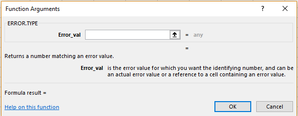
She can give the necessary details and click ‘OK’ to proceed.