Classification Problems and Logistic Regression

Classification Problems

Classification problems are one of the types of problems in which the variable that we want to predict is valued.So we will learn an algorithm called logistic regression which is widely used and one of the most popular learning algorithm.

Here are some examples of classification problems.

To check weather an email is spam or not spam?
To check weather an online transaction is fraudulent or not?

So as you can see the value we want to predict( value of y) may take only two values either ‘0’ or ‘1’ [ 0 for negative class and 1 for positive class].

So for now we will just talk about classification problems with classes 0 and 1, later on we will talk about multi class problems where variable y may take on four values [0,1,2,3] which is called multi class classification problem.

To solve classification problems we can use linear regression as a method in which we can map all predictions greater than 0.5 as a 1 and all less than 0.5 as a 0.However this method is not significant because classification is not actually linear function.

Hypothesis Representation

In this we will see how to represent hypothesis function when we have a classification problem.We can change our hypothesis function to satisfy $0 \leq h_{θ} (x) \leq 1$ . This conditions we can achieved by plugging θTx into the logistic function.

So our new hypothesis function which we achieved by plugging that will use “sigmoid function” or “logistic function” which is represented as following:

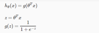
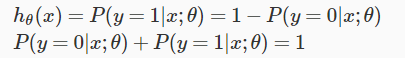
Some in logistic regression $h_{θ} (x)$ will give us the probability that our output is 1.

Decision Boundry

Decision boundry will give us a sense that how will logistic regression’s hypothesis function is computing.

We will translate the output of our hypothesis function as following,in order to get our discrete 0 or 1 classification.

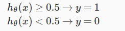
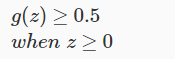
The output of our logistic function is greater then 0.5 whenevar we have our z as greater then or equal to 0 as following:

You can remember the following values of our logistic function which can help us out in future.

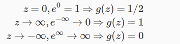
Now because we have input to logistic function as θTX, we will have

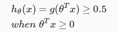
So we lead to this following final conclusion from all this statements:

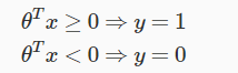
So we will use decision boundry as a line to separate out areas where we have y=1 or where we have y=0.

Cost Function

In this section we will see how we can take the parameters θ for logistic regression. The earlier cost function which we suggested for linear regression will not fit for logistic regression.So we will define a new cost function for logistic regression as following:

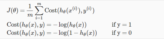
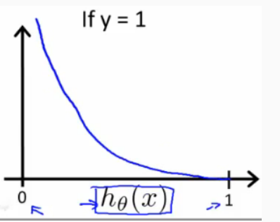
So we have following plot for cost function when y=1.

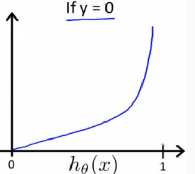
and following plot if we have y=0.

So based on different conditions we have following values for cost function.

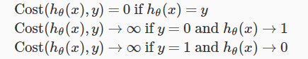
If the value which we want to predict[‘y’] is 0 and if the hypothesis function also outputs 0 then our cost function will have value 0[which can be seen from the figure when y=0]. When our hypothesis function goes towards infinity then our cost function will also approach towards infinity.

If the value which we want to predict[‘y’] is 1 and if the hypothesis function also outputs 1 then our cost function will have value 0[which can be seen from the figure when y=1]. When our hypothesis function goes towards 0 then our cost function will approach towards infinity.

This is all about classification problems and logistic regression algorithm for them.

Join Telegram for Updates